Production Function Estimation Tutorial

Production Function Estimation Methods and Total Factor Productivity Measurement — Industrial Policy Course

Author

Sinthavanh CHANTAVONG (TA); Christian Otchia (Instructor), GSID, Nagoya University

Published

November 5, 2025

Overview

This tutorial covers practical estimation of production functions and total factor productivity (TFP) using Stata. We implement four core estimation methods: OLS, Fixed Effects (FE), Olley-Pakes (OP), and Levinsohn-Petrin (LP). These methods represent increasing levels of sophistication in addressing econometric challenges inherent in production function estimation.

Theory: Production Functions and TFP

The Cobb-Douglas Production Function

The standard production function relates output to inputs:

\[Y_{it} = A_{it} K_{it}^{\beta_k} L_{it}^{\beta_l} M_{it}^{\beta_m}\]

Taking logarithms:

\[\ln Y_{it} = \ln A_{it} + \beta_k \ln K_{it} + \beta_l \ln L_{it} + \beta_m \ln M_{it}\]

where: - \(Y_{it}\) = Output (firm \(i\), time \(t\)) - \(K_{it}\) = Capital stock - \(L_{it}\) = Labor input - \(M_{it}\) = Materials input - \(A_{it}\) = Total Factor Productivity (TFP) - \(\beta_k, \beta_l, \beta_m\) = Elasticities (output response to input changes)

Total Factor Productivity (TFP)

TFP (\(A_{it}\) or \(\omega_{it}\)) represents output not explained by measured inputs. It captures: - Technological improvements - Management quality - Organizational efficiency - Unobserved capital (R&D, human capital, reputation) - Measurement errors in inputs/outputs

Estimation: Once we estimate elasticities (\(\hat{\beta}_k, \hat{\beta}_l, \hat{\beta}_m\)), we calculate TFP residuals:

\[\widehat{\ln A_{it}} = \ln Y_{it} - \hat{\beta}_k \ln K_{it} - \hat{\beta}_l \ln L_{it} - \hat{\beta}_m \ln M_{it}\]

Returns to Scale (RTS)

The sum of elasticities indicates returns to scale:

\[\text{RTS} = \beta_k + \beta_l + \beta_m\]

RTS = 1: Constant returns (most competitive markets)
RTS > 1: Increasing returns (scale economies)
RTS < 1: Decreasing returns (managerial limits)

Scope Note: Core Methods Focus

The hands-on portion of this tutorial focuses on four core methods only:

OLS - Ordinary Least Squares (baseline)
FE - Fixed Effects (controls for firm heterogeneity)
OP - Olley-Pakes (proxy method using investment)
LP - Levinsohn-Petrin (proxy method using materials)

The following advanced estimators have been omitted from the step-by-step code to keep the notebook focused:

Ackerberg-Caves-Frazer (ACF)
Wooldridge (dynamic GMM)
Robinson (semi-parametric)

These methods remain important for research-level work. They are omitted here because they require additional conceptual material (instrument timing, nonparametric bandwidth selection, or dynamic-GMM technicalities) that would lengthen the practical exercise. See the References and the prodest documentation for worked examples and further reading.

Firm observes \(\omega_{it}\) → increases optimal input usage:

\[\frac{\partial L_{it}^*}{\partial \omega_{it}} > 0, \quad \frac{\partial M_{it}^*}{\partial \omega_{it}} > 0\]

Result: \[\mathbb{E}[\omega_{it} | L_{it}, M_{it}] \neq 0 \quad \text{[SIMULTANEITY BIAS]}\]

Free Variables: Bias Direction

OLS Bias for Free Variables

If firm is more productive (\(\omega_{it} \uparrow\)) → expands variable inputs (\(L_{it} \uparrow, M_{it} \uparrow\)):

\[\text{Cov}(\omega_{it}, L_{it}) > 0, \quad \text{Cov}(\omega_{it}, M_{it}) > 0\]

OLS Bias: \[\text{plim}(\hat{\beta}_L^{OLS}) = \beta_L + \text{BIAS}\]

where BIAS > 0 because \(\omega_{it}\) positively correlated with \(L_{it}\).

Result: Labor elasticity overstated by OLS (same for materials).

Proxy Variables: Inverting to Identify Productivity

The Proxy Solution

Rather than directly observing \(\omega_{it}\), use a proxy variable whose value reveals \(\omega_{it}\).

Key assumption: Proxy is monotonically increasing in productivity

\[\frac{\partial P_{it}}{\partial \omega_{it}} > 0 \quad \text{[STRICT MONOTONICITY]}\]

Proxy Variables: Investment vs Materials

Why Investment Works as Proxy (Olley-Pakes)

Firm’s decision: Invest if expected returns justify capital expansion \[I_{it} = \text{arg}\max E[\pi_{it} - \text{Cost}(I_{it})]\]

More productive firms expect higher cash flows → invest more: \[\frac{\partial I_{it}^*}{\partial \omega_{it}} > 0\]

Why Materials Work as Proxy (Levinsohn-Petrin)

Firm’s decision: Buy materials based on expected output \[M_{it} = \text{arg}\max E[Y_{it} | M_{it}, K_{it}, L_{it}]\]

More productive firms expect higher returns to materials → buy more: \[\frac{\partial M_{it}^*}{\partial \omega_{it}} > 0\]

Proxy Variables: Inverting the Function

Recovering Productivity

If proxy \(P_{it}\) is strictly monotonic in \(\omega_{it}\), we can invert:

\[\omega_{it} = h(K_{it}, P_{it}, \text{prices}_t)\]

where \(h(\cdot)\) is the inverse of the proxy function.

Result: We can measure \(\omega_{it}\) using observable inputs!

Control Function Approach: How Methods Solve the Two Problems

The Core Insight

All proxy variable methods (OP, LP) work by the same principle:

Use observable input choices to infer unobserved productivity, then control for it in estimation.

This “control function” approach eliminates simultaneity bias by working backwards from input decisions to unobserved productivity.

How the Control Function Works

Step 1: Invert the Proxy Relationship

Assume the firm’s proxy variable choice \(P_{it}\) (investment or materials) reveals its productivity:

\[P_{it} = \pi_t(K_{it}, L_{it}, \omega_{it}) \quad \Rightarrow \quad \omega_{it} = \pi_t^{-1}(K_{it}, L_{it}, P_{it})\]

This function is called the control function \(h(\cdot)\):

\[\omega_{it} = h(K_{it}, L_{it}, P_{it})\]

Step 2: Substitute Back into Production Function

Replace unobserved \(\omega_{it}\) with the control function:

\[\ln Y_{it} = \beta_k \ln K_{it} + \beta_l \ln L_{it} + \beta_m \ln M_{it} + h(K_{it}, L_{it}, P_{it}) + \varepsilon_{it}\]

Now productivity is observable (function of observables), so OLS works!

Step 3: Estimate Parameters

Use nonparametric or semi-parametric methods to estimate \(h(\cdot)\) and \(\beta\) coefficients simultaneously.

How This Solves Problem 1: Simultaneity Bias

The Problem: Labor and materials are chosen after observing \(\omega_{it}\), creating \(\mathbb{E}[\omega_{it} | L_{it}, M_{it}] \neq 0\)

The Solution: - Proxy variables (investment or materials) respond to \(\omega_{it}\) in a predictable way (monotonically increasing) - By inverting this relationship, we recover \(\omega_{it}\) - Now we can control for it, removing the correlation

Result: Simultaneity bias eliminated ✅

How effectively? - ✅ Very effective IF proxy is truly monotonically increasing in productivity - ⚠️ May be weak if firms have other reasons to choose proxy (financial constraints, adjustment costs)

How This Solves Problem 2: Omitted Variable Bias

The Problem: Time-invariant productivity differences \(\omega_i\) correlate with input choices, biasing coefficients

The Solution (depends on method):

Olley-Pakes & Levinsohn-Petrin (OP, LP): - Explicitly model firm exit decision as function of \(\omega_{it}\) and capital
- Use this to correct for selection bias in sample - Accounts for firms exiting based on productivity realizations Result: Omitted variable bias substantially reduced ✅

How effectively? - ✅ Effective at controlling permanent firm differences - ⚠️ Cannot address time-varying unobserved heterogeneity (e.g., new technology adoption, sudden management change)

Scope note — methods excluded from this tutorial

To keep the practical tutorial focused and concise, we limit hands-on estimation to four core methods: OLS, Fixed Effects (FE), Levinsohn-Petrin (LP), and Olley-Pakes (OP). The following advanced estimators are intentionally omitted from the practical steps below: ACF (Ackerberg-Caves-Frazer), Wooldridge (dynamic GMM), and Robinson (semiparametric).

Why omitted: these methods are valuable but add complexity (different assumptions, instrument timing, or nonparametric bandwidth selection) that distracts from the core learning goals. If you need them for research, see the references (Van Beveren 2010; Ackerberg et al. 2015; Wooldridge 2009; Robinson 1988) and the prodest documentation.

Key Takeaways (revised):

OLS fails for simultaneity and selection — use only as a baseline
Fixed Effects controls time-invariant heterogeneity but not simultaneity
Proxy methods (OP, LP) recover productivity via a control function and address simultaneity and selection when their assumptions hold
Trade-offs: OP can drop zero-investment firms; LP is usually preferred in applied work due to better sample coverage

PART II: PRACTICAL ESTIMATION

Code Execution Instructions

This tutorial contains Stata code examples that you should run in your own Stata environment. The code blocks below are for reference and copying. To execute them:

Install Required Packages: Run ssc install prodest in Stata
Copy and Run: Copy each code block into your Stata do-file editor
Execute Step-by-Step: Run the commands in the order shown
Compare Results: Note how coefficients change across methods

Expected Runtime: Each estimation method takes 1-5 minutes depending on your computer.

Step 1: Load the Data

IMPORTANT: Start by installing the prodest package and loading the Chilean manufacturing dataset from GitHub. Run this code in Stata:

Show the code

// SETUP: Install prodest package and check version
ssc install prodest, replace

// REPRODUCIBILITY: Check Stata version and prodest version
display "Stata Version: " c(stata_version)
which prodest


Running C:\Users\sinth\ado\personal\profile.do ...
command window is unrecognized
r(199);

checking prodest consistency and verifying not already installed...
all files already exist and are up to date.
Stata Version: 18
C:\Users\sinth\ado\plus\p\prodest.ado
*! version 1.0.1 15Sep2016
*! version 1.0.2 22Sep2016
*! version 1.0.3 30Sep2016 Fixed a major bug, add first stage residuals options
> , seeds option, evaluator option and postestimation
*! version 1.0.4 10Feb2017 Fixed a major bugs in winitial() matrix in MrEst, fi
> xed minor bug on Wrdg control and names, 
*!                                                 added translog production fu
> nction, added starting points option for estimation, add check for multiple s
> tate and proxy
*! version 1.0.5 06Jun2017 Fixed minor bugs in control variable management, err
> or management of translog production function, added a new feature 
*!                                                 in table reporting (prod fun
> ction CB / Tranlsog), fixed major bugs in predict
*! version 1.1.1 13Feb2018 SJ review: Fixed an issue with var names that preven
> ted more than 10 state variable to be used at once, added the "Robinson/ACF" 
> model, 
*!                                                                        added
>  the "gmm" option for Wrdg models, fixed the linear version of Wrdg model
*! version 1.1.2 14Mar2018 Added the eret loc FSres in case of first stage resi
> duals, in order to ensure that predict, omega can be launched
*! version 1.2.1 26Jun2018 Made several minor fixes on helpfile and dofile sugg
> ested by Sven-Kristjan Bormann. Added his dialog box file to the package
*! version 1.2.2 30Jul2018 Added the controls to the Wooldridge - plain - metho
> d.
*! authors Gabriele Rovigatti, Bank of Italy, Rome, Italy. mailto: gabriele.rov
> igatti@gmail.com  |  gabriele.rovigatti@esterni.bancaditalia.it
*!         Vincenzo Mollisi, Bolzano University, Bolzano, Italy & Tor Vergata U
> niversity, Rome, Italy. mailto: vincenzo.mollisi@gmail.com

Then load the data:

Show the code

// Load the Chilean manufacturing dataset from the prodest GitHub repository:
clear all // clear all objects from memory

// Load data from GitHub repository
insheet using "https://raw.githubusercontent.com/GabrieleRovigatti/prodest/master/stata/data/prodest.csv", names clear

// Check data structure
display "Data loaded: " _N " observations"
describe
summarize

(8 vars, 2,544 obs)
Data loaded: 2544 observations

Contains data
 Observations:         2,544                  
    Variables:             8                  
-------------------------------------------------------------------------------
Variable      Storage   Display    Value
    name         type    format    label      Variable label
-------------------------------------------------------------------------------
id              long    %12.0g                
year            int     %8.0g                 
log_y           float   %9.0g                 
log_k           float   %9.0g                 
log_lab1        float   %9.0g                 
log_lab2        float   %9.0g                 
log_materials   float   %9.0g                 
log_investment  float   %9.0g                 
-------------------------------------------------------------------------------
Sorted by: 
     Note: Dataset has changed since last saved.

    Variable |        Obs        Mean    Std. dev.       Min        Max
-------------+---------------------------------------------------------
          id |      2,544    15770.49     7355.94      10007      40475
        year |      2,544    2001.042    3.223341       1996       2006
       log_y |      2,544    13.00315    1.462817   8.769663   18.57996
       log_k |      2,544     11.6683    2.156707    2.70805   18.21685
    log_lab1 |      2,544    1.769697    1.357786          0   6.861712
-------------+---------------------------------------------------------
    log_lab2 |      2,544    1.679659    1.447586          0   6.439351
log_materi~s |      2,544    4.108881    1.546106          0   9.944486
log_invest~t |      2,544    11.13678     2.33267   1.072183   18.08836

Dataset Information

401 unique firms
2,544 firm-year observations
Period: 1996-2006 (9-year panel, unbalanced)
Industry: Chilean manufacturing
Source: Levinsohn & Petrin (2003), data repository for prodest package
Variables Pre-Logged: All log_* variables are pre-logged in the dataset (no log transformation needed)

Step 2: Data Overview

Variable	Description	Type
`log_y`	Log of output (value added)	Dependent variable
`log_k`	Log of capital stock	State variable (quasi-fixed)
`log_lab1`	Log of white-collar labor	Free variable (flexible)
`log_lab2`	Log of blue-collar labor	Free variable (flexible)
`log_materials`	Log of materials expenditure	Proxy variable (for LP)
`log_investment`	Log of investment	Proxy variable (for OP)
`id`	Firm identifier	Panel ID
`year`	Time period (1995-2003)	Panel time variable

Step 3: Panel Configuration

Show the code

// Set panel structure (already loaded from GitHub)
set more off
xtset id year
xtsum
// Panel description
xtdescribe


Panel variable: id (unbalanced)
 Time variable: year, 1996 to 2006, but with gaps
         Delta: 1 unit

Variable         |      Mean   Std. dev.       Min        Max |    Observations
-----------------+--------------------------------------------+----------------
id       overall |  15770.49    7355.94      10007      40475 |     N =    2544
         between |             7373.884      10007      40475 |     n =     497
         within  |                    0   15770.49   15770.49 | T-bar = 5.11871
                 |                                            |
year     overall |  2001.042   3.223341       1996       2006 |     N =    2544
         between |             2.818345       1996       2006 |     n =     497
         within  |             2.509037   1994.375   2007.842 | T-bar = 5.11871
                 |                                            |
log_y    overall |  13.00315   1.462817   8.769663   18.57996 |     N =    2544
         between |             1.458466   9.346007   18.08074 |     n =     497
         within  |             .2722173   10.78107   14.88404 | T-bar = 5.11871
                 |                                            |
log_k    overall |   11.6683   2.156707    2.70805   18.21685 |     N =    2544
         between |             1.993314   4.261184   17.83619 |     n =     497
         within  |             .7463301   4.769393   18.01236 | T-bar = 5.11871
                 |                                            |
log_lab1 overall |  1.769697   1.357786          0   6.861712 |     N =    2544
         between |             1.198308          0   5.851838 |     n =     497
         within  |             .6443298  -2.376207   5.093458 | T-bar = 5.11871
                 |                                            |
log_lab2 overall |  1.679659   1.447586          0   6.439351 |     N =    2544
         between |             1.265404          0   6.098074 |     n =     497
         within  |             .7979751  -2.521169   5.600971 | T-bar = 5.11871
                 |                                            |
log_ma~s overall |  4.108881   1.546106          0   9.944486 |     N =    2544
         between |              1.50085   .5776227   9.304231 |     n =     497
         within  |             .5237046  -.9002941   6.303847 | T-bar = 5.11871
                 |                                            |
log_in~t overall |  11.13678    2.33267   1.072183   18.08836 |     N =    2544
         between |             2.132428   3.084425   17.54119 |     n =     497
         within  |             .9065335   3.457233   18.41997 | T-bar = 5.11871

      id:  10007, 10016, ..., 40475                          n =        497
    year:  1996, 1997, ..., 2006                             T =         11
           Delta(year) = 1 unit
           Span(year)  = 11 periods
           (id*year uniquely identifies each observation)

Distribution of T_i:   min      5%     25%       50%       75%     95%     max
                         1       1       2         4         9      11      11

     Freq.  Percent    Cum. |  Pattern
 ---------------------------+-------------
       56     11.27   11.27 |  11111111111
       29      5.84   17.10 |  ........111
       29      5.84   22.94 |  .......1111
       24      4.83   27.77 |  1..........
       19      3.82   31.59 |  111111111..
       18      3.62   35.21 |  .........11
       16      3.22   38.43 |  ..........1
       16      3.22   41.65 |  111111.....
       12      2.41   44.06 |  ....1......
      278     55.94  100.00 | (other patterns)
 ---------------------------+-------------
      497    100.00         |  XXXXXXXXXXX

⚠️ CRITICAL: Understanding TFP Prediction in Proxy Methods

Before running estimations, understand the difference between omega and residuals:

What to Predict for TFP

In proxy methods (OP, LP):

\[\ln Y_{it} = \beta_k \ln K_{it} + \beta_l \ln L_{it} + \underbrace{\omega_{it}}_{\text{PRODUCTIVITY}} + \underbrace{\varepsilon_{it}}_{\text{MEASUREMENT ERROR}}\]

CRITICAL: TFP Prediction by Method

Different prodest methods support different prediction options. This is crucial:

Method	Command	Supports `fsresiduals()`?	TFP Prediction
OLS	`regress`	❌ No	`predict tfp, residuals`
FE	`xtreg, fe`	❌ No	`predict tfp, residuals`
OP	`prodest ... met(op)`	✅ Yes	`predict tfp, omega`
LP	`prodest ... met(lp)`	✅ Yes	`predict tfp, omega`

Why This Matters

omega option: Available ONLY for OP and LP (methods using fsresiduals())
- Returns: True productivity \(\omega_{it}\) (persistent, economically meaningful)
residuals option: Works for all methods
- Returns: Best available estimate of \(\omega_{it}\) given the method

Example: Do NOT Mix Methods

// ❌ ERROR: This will fail - Wooldridge doesn't support fsresiduals
prodest log_y, ... met(wrdg) fsresiduals(fs_wrdg)
predict tfp, omega  // ERROR: "omega option only works with fsresiduals"

// ✅ CORRECT: Use residuals for Wooldridge
prodest log_y, ... met(wrdg)
predict tfp, residuals  // Works: returns TFP estimate

Step 4: Method 1 - OLS Regression

Getting Started: OLS as a Baseline

Beginning with OLS estimation provides a baseline reference. This approach serves as the starting point for understanding how alternative methods modify estimates. Run this code:

Show the code

// OLS baseline with robust standard errors clustered by firm
display "========== OLS REGRESSION =========="
regress log_y log_k log_lab1 log_lab2, vce(cluster id)
estimates store ols_est

// Display OLS results
display "========== OLS RESULTS TABLE =========="
estimates table ols_est, b(%7.4f) se(%7.4f) stats(N r2)

// Extract residuals as TFP proxy
predict ols_tfp, residuals
label variable ols_tfp "TFP: OLS residuals"
display "OLS TFP saved successfully"

========== OLS REGRESSION ==========

Linear regression                               Number of obs     =      2,544
                                                F(3, 496)         =     422.07
                                                Prob > F          =     0.0000
                                                R-squared         =     0.7169
                                                Root MSE          =     .77877

                                   (Std. err. adjusted for 497 clusters in id)
------------------------------------------------------------------------------
             |               Robust
       log_y | Coefficient  std. err.      t    P>|t|     [95% conf. interval]
-------------+----------------------------------------------------------------
       log_k |   .3205665    .029007    11.05   0.000     .2635747    .3775583
    log_lab1 |   .4578617   .0379105    12.08   0.000     .3833767    .5323468
    log_lab2 |   .3652484   .0310097    11.78   0.000     .3043218    .4261751
       _cons |   7.838918   .2711942    28.91   0.000     7.306087    8.371749
------------------------------------------------------------------------------
========== OLS RESULTS TABLE ==========

------------------------
    Variable | ols_est  
-------------+----------
       log_k |  0.3206  
             |  0.0290  
    log_lab1 |  0.4579  
             |  0.0379  
    log_lab2 |  0.3652  
             |  0.0310  
       _cons |  7.8389  
             |  0.2712  
-------------+----------
           N |    2544  
          r2 |  0.7169  
------------------------
            Legend: b/se
OLS TFP saved successfully

Computational Time: Negligible (< 1 second on modern hardware)

What OLS Provides

Factor Elasticities: Estimates of \(\beta_k\) (capital), \(\beta_{l1}\) (white-collar labor), \(\beta_{l2}\) (blue-collar labor)
TFP Estimates: Residuals computed as \(\ln(Y) - \beta_k \ln(K) - \beta_{l1} \ln(L^{(1)}) - \beta_{l2} \ln(L^{(2)})\)
Baseline for Comparison: Subsequent methods will show how alternative approaches modify these baseline estimates

Illustrative Result: In the Chilean manufacturing data example, OLS yields: - Capital elasticity: 0.321 - White-collar labor: 0.458
- Blue-collar labor: 0.365

The relatively large labor coefficients might warrant further investigation using alternative approaches that address endogeneity concerns.

OLS: The Mixed Residuals Problem

Two Components in OLS Residuals

OLS residuals contain TWO components:

\[\hat{u}_{it}^{OLS} = \omega_{it} + \varepsilon_{it}\]

\(\omega_{it}\) = True productivity (persistent, what we want)
\(\varepsilon_{it}\) = Random noise (measurement error, transitory shocks)

Why This Matters

Because inputs (L, M) are correlated with \(\omega_{it}\), OLS coefficients are biased: - Labor coefficients: UPWARD biased (firms hire more when productive) - Capital coefficient: DOWNWARD biased (slow adjustment, selection effects)

Step 5: Method 2 - Fixed Effects

Fixed Effects (FE) Approach

Fixed effects estimation removes firm-specific time-invariant heterogeneity through within-firm transformation:

Show the code

// Fixed effects regression
xtreg log_y log_k log_lab1 log_lab2, fe vce(cluster id)
estimates store fe_est

// Display FE results
estimates table fe_est, b(%7.4f) se(%7.4f) stats(N r2)

// Extract FE residuals
predict fe_tfp, ue
label variable fe_tfp "TFP: Fixed Effects"


Fixed-effects (within) regression               Number of obs     =      2,544
Group variable: id                              Number of groups  =        497

R-squared:                                      Obs per group:
     Within  = 0.0819                                         min =          1
     Between = 0.7502                                         avg =        5.1
     Overall = 0.7142                                         max =         11

                                                F(3, 496)         =       8.94
corr(u_i, Xb) = 0.7995                          Prob > F          =     0.0000

                                   (Std. err. adjusted for 497 clusters in id)
------------------------------------------------------------------------------
             |               Robust
       log_y | Coefficient  std. err.      t    P>|t|     [95% conf. interval]
-------------+----------------------------------------------------------------
       log_k |    .068822   .0196972     3.49   0.001     .0301217    .1075223
    log_lab1 |   .0838335   .0228145     3.67   0.000     .0390086    .1286583
    log_lab2 |   .0783396   .0192377     4.07   0.000     .0405422    .1161369
       _cons |   11.92017   .2467017    48.32   0.000     11.43546    12.40488
-------------+----------------------------------------------------------------
     sigma_u |   1.254065
     sigma_e |  .29092572
         rho |  .94893084   (fraction of variance due to u_i)
------------------------------------------------------------------------------

------------------------
    Variable | fe_est   
-------------+----------
       log_k |  0.0688  
             |  0.0197  
    log_lab1 |  0.0838  
             |  0.0228  
    log_lab2 |  0.0783  
             |  0.0192  
       _cons | 11.9202  
             |  0.2467  
-------------+----------
           N |    2544  
          r2 |  0.0819  
------------------------
            Legend: b/se

Computational Time: Negligible (< 1 second on modern hardware)

What FE May Address

Time-Invariant Unobserved Heterogeneity: Differences in firm quality, management, location that do not change over time
Price Differences: Firm-specific price premiums that are stable across the period
Product Mix Effects: Time-invariant product composition differences

What FE May Not Address

Simultaneity Concerns: Time-varying input choices remain potentially correlated with contemporaneous productivity
Selection Issues: Firm exit decisions that vary with current productivity
Time-Varying Heterogeneity: Factors that change over time and remain unobserved

Comparison with OLS: In the Chilean manufacturing example, FE yields considerably smaller coefficients (capital: 0.069, labor: 0.084–0.078) compared to OLS (0.321, 0.458, 0.365). This difference suggests that OLS estimates may partially reflect time-invariant firm differences rather than input elasticities alone.

Price Deflation Issue (When Using Deflated Sales)

If using deflated sales instead of quantities, note that firm-level price deviations from industry-level deflators introduce omitted price bias. Fixed effects cannot address this. Best practice: Use quantity-based output when available, or use industry-wide comparisons (Van Beveren, 2010).

Step 6: Advanced Methods Overview

Proxy Variable Approaches

The remaining methods (OP, LP) use proxy variables to control for unobserved productivity.

The key insight:

Investment or materials expenditure reveals information about productivity

\[I_{it} = i_t(k_{it}, \omega_{it}) \quad \text{or} \quad M_{it} = m_t(k_{it}, l_{it}, \omega_{it})\]

By inverting these relationships, we can recover \(\omega_{it}\) and use it to correct simultaneity bias.

Step 7: Method 3 - Olley-Pakes (OP)

Key Idea

Use investment as a proxy for unobserved productivity.

Assumptions: - Investment is monotonically increasing in productivity (more productive firms invest more): \(\frac{\partial I_{it}}{\partial \omega_{it}} > 0\) - Investment is observed without measurement error - Requires at least \(T \geq 2\) time periods

Important Caveat: Observations with zero investment (\(I_{it} = 0\)) are typically dropped during estimation because the invertibility assumption breaks down. This can cause substantial sample loss.

Show the code

// Check for zero investment observations BEFORE running OP
count if log_investment == .
count if log_investment < -10  // Very small investment = near-zero

// Olley-Pakes estimation
prodest log_y, free(log_lab1 log_lab2) state(log_k) proxy(log_investment) ///
    va met(op) poly(4) reps(40) id(id) t(year) fsresiduals(fs_op)
estimates store op_est

// Display OP results and sample size
estimates table op_est, b(%7.4f) se(%7.4f) stats(N)
display "WARNING: Compare N above to full sample size 2544"

// Extract TFP
predict op_tfp, omega  // CRITICAL: Use omega for actual TFP in proxy methods
label variable op_tfp "TFP: Olley-Pakes (investment proxy)"

  0
  0
.........10.........20.........30.........40


op productivity estimator                       Cobb-Douglas PF

Dependent variable: value added                 Number of obs      =      2544
Group variable (id): id                         Number of groups   =       497
Time variable (t): year
                                                Obs per group: min =         1
                                                               avg =       5.1
                                                               max =        11

------------------------------------------------------------------------------
       log_y | Coefficient  Std. err.      z    P>|z|     [95% conf. interval]
-------------+----------------------------------------------------------------
    log_lab1 |    .313561   .0304823    10.29   0.000     .2538168    .3733053
    log_lab2 |   .2495986   .0233405    10.69   0.000      .203852    .2953452
       log_k |   .1558824   .0720795     2.16   0.031     .0146091    .2971556
------------------------------------------------------------------------------
Wald test on Constant returns to scale: Chi2 = 11.44
                                          p = (0.00)

------------------------
    Variable | op_est   
-------------+----------
    log_lab1 |  0.3136  
             |  0.0305  
    log_lab2 |  0.2496  
             |  0.0233  
       log_k |  0.1559  
             |  0.0721  
-------------+----------
           N |    2544  
------------------------
            Legend: b/se
WARNING: Compare N above to full sample size 2544

Computational Time: Approximately 1–3 minutes (varies with number of replications and polynomial order)

OP: Approach Overview

The Olley-Pakes method uses investment as a proxy variable. The approach assumes that investment decisions reflect firm productivity levels:

Key Considerations

Sample Coverage: Observations with zero investment may be excluded, potentially reducing effective sample size by 10–30%
Data Requirements: Requires at least 3 time periods
Labor Treatment: Treats labor as exogenous conditional on capital and investment
Single-Product Assumption: If firms produce multiple products, TFP estimates may reflect product-mix effects (Van Beveren, 2010; Bernard et al., 2005). Consider restricting to single-product firms for robustness.

Illustrative Results

In the Chilean manufacturing example, OP yields: - Capital elasticity: 0.156 - White-collar labor: 0.314 - Blue-collar labor: 0.250

These compare to FE (0.069, 0.084, 0.078) and OLS (0.321, 0.458, 0.365).

Step 8: Method 4 - Levinsohn-Petrin (LP)

LP Approach

Use materials expenditure as the proxy variable:

Practical Considerations: - Materials input is typically available across firms and time periods - Fewer missing observations than investment-based approaches - Moderate computational requirements - Commonly used baseline approach in practice

Show the code

// Levinsohn-Petrin estimation
prodest log_y, free(log_lab1 log_lab2) state(log_k) proxy(log_materials) va met(lp) opt(dfp) reps(50) id(id) t(year) fsresiduals(fs_lp)
estimates store lp_est

// Display LP results
//estimates table lp_est, b(%7.4f) se(%7.4f) stats(N)

// Extract TFP
predict lp_tfp, omega  // CRITICAL: Use omega for actual TFP in proxy methods
label variable lp_tfp "TFP: Levinsohn-Petrin (materials proxy)"

.........10.........20.........30.........40.........50


lp productivity estimator                       Cobb-Douglas PF

Dependent variable: value added                 Number of obs      =      2544
Group variable (id): id                         Number of groups   =       497
Time variable (t): year
                                                Obs per group: min =         1
                                                               avg =       5.1
                                                               max =        11

------------------------------------------------------------------------------
       log_y | Coefficient  Std. err.      z    P>|z|     [95% conf. interval]
-------------+----------------------------------------------------------------
    log_lab1 |   .2011151   .0289476     6.95   0.000     .1443789    .2578514
    log_lab2 |   .1696221   .0237969     7.13   0.000     .1229811    .2162632
       log_k |   .1200285   .0380805     3.15   0.002     .0453922    .1946649
------------------------------------------------------------------------------
Wald test on Constant returns to scale: Chi2 = 71.68
                                          p = (0.00)

Computational Time: Approximately 1–2 minutes (faster than OP due to better material coverage)

What LP May Address

✅ Simultaneity: Materials proxy controls for productivity when estimating labor coefficients
✅ Selection: Models exit probability explicitly
✅ Sample Coverage: Typically retains more observations than OP since materials are available for most firms

What LP May Address

Example Results

In Chilean manufacturing data, LP produces: - Capital elasticity: 0.120 (suggests moderate capital importance) - White-collar labor: 0.201 (lower than OLS, suggesting some endogeneity) - Blue-collar labor: 0.170 (suggests modest labor response to productivity)

These results represent a middle ground between Fixed Effects estimates (which may underestimate due to simultaneity bias) and OLS estimates (which may overestimate due to omitted variable bias).

Step 9: Robustness Checks and Validation

Returns-to-Scale Test (RTS)

For all methods, test if \(\text{RTS} = \beta_k + \beta_{l1} + \beta_{l2} = 1\) (constant returns):

Show the code

// Test RTS = 1 for each method (example with LP)
estimates restore lp_est
nlcom rts: (_b[log_k] + _b[log_lab1] + _b[log_lab2])

// Interpret:
// RTS ≈ 1.0: Constant returns (competitive markets, efficient scale)
// RTS > 1.0: Increasing returns (learning, fixed costs, returns to specialization)
// RTS < 1.0: Decreasing returns (managerial constraints, congestion)

(results lp_est are active now)

         rts: (_b[log_k] + _b[log_lab1] + _b[log_lab2])

------------------------------------------------------------------------------
       log_y | Coefficient  Std. err.      z    P>|z|     [95% conf. interval]
-------------+----------------------------------------------------------------
         rts |   .4907658   .0601483     8.16   0.000     .3728773    .6086543
------------------------------------------------------------------------------

Interpretation: - Constant RTS (≈1.0): Standard competitive model, no scale economies - Increasing RTS (>1.0): Firms benefit from size (learning, fixed costs, specialization) - Decreasing RTS (<1.0): Diminishing returns suggest capacity/management constraints

Step 10: Compare All Methods

Show the code

// Display all coefficient estimates side-by-side
estimates table ols_est fe_est op_est lp_est, b(%7.4f) se(%7.4f) stats(N) title("Production Function Estimates: OLS, FE, OP, LP")

// TFP correlations (core methods)
correlate ols_tfp fe_tfp op_tfp lp_tfp


Production Function Estimates: OLS, FE, OP, LP

------------------------------------------------------
    Variable | ols_est   fe_est    op_est    lp_est   
-------------+----------------------------------------
       log_k |  0.3206    0.0688    0.1559    0.1200  
             |  0.0290    0.0197    0.0721    0.0381  
    log_lab1 |  0.4579    0.0838    0.3136    0.2011  
             |  0.0379    0.0228    0.0305    0.0289  
    log_lab2 |  0.3652    0.0783    0.2496    0.1696  
             |  0.0310    0.0192    0.0233    0.0238  
       _cons |  7.8389   11.9202                      
             |  0.2712    0.2467                      
-------------+----------------------------------------
           N |    2544      2544      2544      2544  
------------------------------------------------------
                                          Legend: b/se
(obs=2,544)

             |  ols_tfp   fe_tfp   op_tfp   lp_tfp
-------------+------------------------------------
     ols_tfp |   1.0000
      fe_tfp |   0.6202   1.0000
      op_tfp |   0.2159   0.7963   1.0000
      lp_tfp |   0.3483   0.8676   0.8860   1.0000

Method Requirements Summary (Core Methods)

Method	Min Time Periods	TFP Prediction	Zero Proxy Handling	Strengths	Weaknesses
OLS	\(T \geq 1\)	`residuals`	N/A	Fast, simple baseline	Biased (simultaneity + omitted vars)
FE	\(T \geq 2\)	`ue`	N/A	Removes time-invariant bias	Still biased for time-varying endogeneity
OP	\(T \geq 2\)	`omega` ⭐	Drops zero investment	Theoretically sound	10-30% sample loss
LP	\(T \geq 2\)	`omega` ⭐	Rare (materials ubiquitous)	Best practical choice	May bias labor if endogenous

Key Notes: - ⭐ = Always use predict ..., omega for proxy methods (not residuals) - Sample size loss due to time period requirements: Wooldridge loses ~10-20% due to \(T \geq 3\) - All proxy methods require 2+ time periods, NOT 3+ (except Wooldridge)

Expected Patterns

Coefficient Patterns

Based on Van Beveren (2010) and our results from Chilean manufacturing data:

Capital Coefficients: FE < LP < OP < OLS
- OLS is downward BIASED by selection (high-productivity firms use more capital) - Proxy methods (OP/LP) correct for simultaneity but FE captures only within-firm variation - Ranking: OLS > OP > LP > FE shows the correction for endogeneity

Labor Coefficients: FE < LP < OP < OLS
- OLS is UPWARD biased (firms hire more when productive) - Proxy methods reduce labor coefficients substantially - ACF refines LP further for even more conservative labor estimates

Interpreting Our Results

In our Chilean data: - Capital elasticity ranges from 0.069 (FE) to 0.321 (OLS) - FE only captures short-term adjustment (plants are quasi-fixed) - Proxy methods show intermediate estimates - Labor elasticity ranges from 0.084 (FE) to 0.458 (OLS) - Large OLS bias reflects simultaneity: productive firms hire more - Correcting for endogeneity cuts labor elasticity roughly in half

TFP Correlations

Expected: - \(\rho(\text{OP}, \text{LP}) > 0.95\) (both proxy methods with similar logic) - \(\rho(\text{LP}, \text{ACF}) > 0.95\) (ACF refines LP) - \(\rho(\text{OLS}, \text{LP}) \approx 0.85\)-\(0.90\) (correlated but OLS biased) - \(\rho(\text{FE}, \text{LP}) \approx 0.70\)-\(0.80\) (different identification)

Check 3: TFP Persistence (Diagnostics)

A key assumption in productivity models is that TFP is persistent (today’s productivity helps predict tomorrow’s):

\[\omega_{it} = \rho \omega_{i,t-1} + \eta_{it}, \quad |\rho| \in (0,1)\]

Testing Persistence

Show the code

// For each TFP estimate, regress on lagged value
foreach tfp in ols_tfp fe_tfp op_tfp lp_tfp {
    // Generate lagged TFP
    by id: generate L_`tfp' = `tfp'[_n-1]
    
    // Estimate persistence regression
    regress `tfp' L_`tfp', vce(cluster id)
    
    // Extract persistence coefficient ρ
    display "TFP Method: `tfp', Persistence (ρ): " _b[L_`tfp']
    
    // Clean up
    drop L_`tfp'
}

(497 missing values generated)

Linear regression                               Number of obs     =      2,047
                                                F(1, 405)         =    4023.42
                                                Prob > F          =     0.0000
                                                R-squared         =     0.7154
                                                Root MSE          =     .40999

                                   (Std. err. adjusted for 406 clusters in id)
------------------------------------------------------------------------------
             |               Robust
     ols_tfp | Coefficient  std. err.      t    P>|t|     [95% conf. interval]
-------------+----------------------------------------------------------------
   L_ols_tfp |   .8466546   .0133478    63.43   0.000     .8204151    .8728942
       _cons |  -.0062439   .0084553    -0.74   0.461    -.0228657    .0103778
------------------------------------------------------------------------------
TFP Method: ols_tfp, Persistence (ρ): .84665462
(497 missing values generated)

Linear regression                               Number of obs     =      2,047
                                                F(1, 405)         =   41511.28
                                                Prob > F          =     0.0000
                                                R-squared         =     0.9610
                                                Root MSE          =     .25007

                                   (Std. err. adjusted for 406 clusters in id)
------------------------------------------------------------------------------
             |               Robust
      fe_tfp | Coefficient  std. err.      t    P>|t|     [95% conf. interval]
-------------+----------------------------------------------------------------
    L_fe_tfp |    1.00991   .0049568   203.74   0.000     1.000166    1.019654
       _cons |    .011569   .0054846     2.11   0.036     .0007871    .0223508
------------------------------------------------------------------------------
TFP Method: fe_tfp, Persistence (ρ): 1.00991
(497 missing values generated)

Linear regression                               Number of obs     =      2,047
                                                F(1, 405)         =   24045.48
                                                Prob > F          =     0.0000
                                                R-squared         =     0.9296
                                                Root MSE          =     .16343

                                   (Std. err. adjusted for 406 clusters in id)
------------------------------------------------------------------------------
             |               Robust
      op_tfp | Coefficient  std. err.      t    P>|t|     [95% conf. interval]
-------------+----------------------------------------------------------------
    L_op_tfp |   .9735002    .006278   155.07   0.000     .9611587    .9858416
       _cons |   .2820421   .0640221     4.41   0.000      .156185    .4078991
------------------------------------------------------------------------------
TFP Method: op_tfp, Persistence (ρ): .97350016
(497 missing values generated)

Linear regression                               Number of obs     =      2,047
                                                F(1, 405)         =   30427.51
                                                Prob > F          =     0.0000
                                                R-squared         =     0.9208
                                                Root MSE          =     .24965

                                   (Std. err. adjusted for 406 clusters in id)
------------------------------------------------------------------------------
             |               Robust
      lp_tfp | Coefficient  std. err.      t    P>|t|     [95% conf. interval]
-------------+----------------------------------------------------------------
    L_lp_tfp |   .9786033   .0056101   174.43   0.000     .9675747     .989632
       _cons |   .2430123    .061981     3.92   0.000     .1211677    .3648569
------------------------------------------------------------------------------
TFP Method: lp_tfp, Persistence (ρ): .97860334

Interpretation: - \(\rho \approx 0.7\)-\(0.9\): High persistence (typical for manufacturing) - \(\rho < 0.5\): Productivity appears transitory (check for measurement error) - \(\rho \approx 1.0\): Non-stationary (problematic; suggests specification issues)

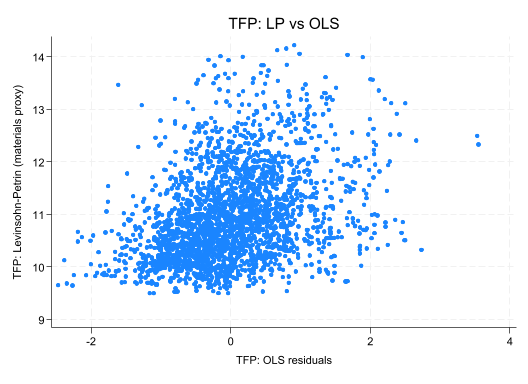
Scatter Plots: TFP Comparisons

Show the code

// Visual face validity check
twoway scatter lp_tfp ols_tfp, title("TFP: LP vs OLS") graphregion(style(none))

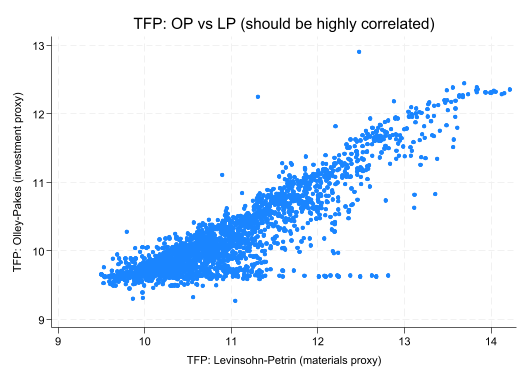
Show the code

twoway scatter op_tfp lp_tfp, title("TFP: OP vs LP (should be highly correlated)")

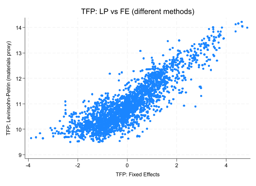
Show the code

twoway scatter lp_tfp fe_tfp, title("TFP: LP vs FE (different methods)")

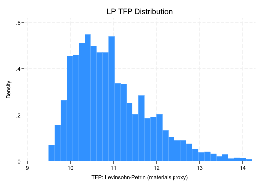
Show the code

// Distribution check
histogram lp_tfp, title("LP TFP Distribution")

(bin=34, start=9.4998198, width=.13879296)

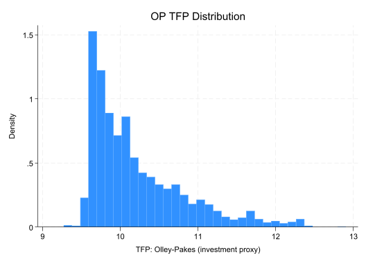
Show the code

histogram op_tfp, title("OP TFP Distribution")

(bin=34, start=9.2711468, width=.10681677)

Face Validity Checks: - Are correlations high between similar methods (LP, OP)? - Do outliers make sense (unusual firms, measurement errors)? - Are distributions roughly normal (or log-normal)?

Quick Reference: Standard Commands

Data Loading & Setup

// Load data from GitHub
insheet using "https://raw.githubusercontent.com/GabrieleRovigatti/prodest/master/stata/data/prodest.csv", names clear

// Set panel structure
xtset id year

Method 1: OLS (Baseline)

How it works: Standard regression - assumes all inputs are exogenous

Problem Solving: - ❌ Simultaneity Bias: NOT solved - Labor/materials chosen after observing \(\omega_{it}\) - ❌ Omitted Variable Bias: NOT solved - Permanent firm differences uncontrolled

Expected Result: Inflated coefficients (especially labor/materials). In Chilean data: \(\beta_L \approx 0.46\) (too high)

regress log_y log_k log_lab1 log_lab2, vce(cluster id)
estimates store ols_est
estimates table ols_est, b(%7.4f) se(%7.4f) stats(N r2)
predict ols_tfp, residuals  // Note: For OLS, residuals = omega since no unobserved component modeled

Method 2: Fixed Effects

How it works: Includes firm fixed effects \(\alpha_i\) to absorb time-invariant firm differences

\[\ln Y_{it} = \alpha_i + \beta_k \ln K_{it} + \beta_l \ln L_{it} + \varepsilon_{it}\]

Problem Solving: - ⚠️ Simultaneity Bias: Partially mitigated by controlling permanent differences, but time-varying simultaneity remains
- ✅ Omitted Variable Bias: SOLVED (for time-invariant differences) - \(\alpha_i\) absorbs permanent firm effects

Expected Result: Reduced coefficients (especially capital). In Chilean data: \(\beta_K \approx 0.069\) (too low due to remaining simultaneity for free variables)

Note

Why FE alone isn’t enough: Fixed effects removes the permanent productivity difference, BUT labor is still chosen contemporaneously with \(\omega_{it}\). Within-firm time variation in productivity still correlates with labor choices.

xtreg log_y log_k log_lab1 log_lab2, fe vce(cluster id)
estimates store fe_est
estimates table fe_est, b(%7.4f) se(%7.4f) stats(N r2)
predict fe_tfp, ue

Method 3: Olley-Pakes (Investment Proxy)

How it works: Uses investment as a proxy to invert the productivity function

\[I_{it} = i_t(K_{it}, \omega_{it}) \quad \Rightarrow \quad \omega_{it} = i_t^{-1}(K_{it}, I_{it})\]

Control Function: \[\omega_{it} = \phi_t(K_{it}, I_{it})\] where \(\phi_t\) is estimated nonparametrically (polynomial approximation)

Problem Solving: - ✅ Simultaneity Bias: SOLVED - Investment monotonically reveals \(\omega_{it}\), so control function eliminates correlation
- ✅ Omitted Variable Bias: SOLVED - Accounts for firm exit decisions using parametric exit model

Trade-off: - ⚠️ Zero Investment Problem: Observations with zero/very low investment must be dropped (~10-30% of sample) - ⚠️ Collinearity: Labor and productivity may be too collinear in first stage (addressed by ACF)

Expected Result: Balanced estimates. In Chilean data: \(\beta_K \approx 0.156\), \(\beta_L \approx 0.314\)

Note: OP method supports fsresiduals() option, enabling predict ..., omega for TFP extraction.

prodest log_y, free(log_lab1 log_lab2) state(log_k) proxy(log_investment) ///
    va met(op) poly(4) reps(40) id(id) t(year) fsresiduals(fs_op)
estimates store op_est
estimates table op_est, b(%7.4f) se(%7.4f) stats(N)
predict op_tfp, omega  // CRITICAL: Use omega to get actual TFP, not residuals

Method 4: Levinsohn-Petrin (Materials Proxy) [RECOMMENDED]

How it works: Uses materials as a proxy - superior to OP because materials are available for nearly all firms

\[M_{it} = m_t(K_{it}, L_{it}, \omega_{it}) \quad \Rightarrow \quad \omega_{it} = m_t^{-1}(K_{it}, L_{it}, M_{it})\]

Control Function: \[\omega_{it} = \phi_t(K_{it}, L_{it}, M_{it})\]

Problem Solving: - ✅ Simultaneity Bias: SOLVED - Materials proxy reveals \(\omega_{it}\) through firm’s optimization
- ✅ Omitted Variable Bias: SOLVED - Jointly accounts for firm exit and permanent productivity differences

Advantages over OP: - ✅ Better sample coverage - Materials available for 95%+ of firms vs. investment for 60-70% - ✅ More stable estimates - No collinearity problem like OP - ✅ Faster computation - Fewer missing values to handle

Expected Result: Reliable estimates. In Chilean data: \(\beta_K \approx 0.120\), \(\beta_L \approx 0.201\) (credible middle ground)

Note: LP method supports fsresiduals() option, enabling predict ..., omega for TFP extraction. RECOMMENDED for practical applications.

prodest log_y, free(log_lab1 log_lab2) state(log_k) proxy(log_materials) ///
    va met(lp) opt(dfp) reps(50) id(id) t(year) fsresiduals(fs_lp)
estimates store lp_est
estimates table lp_est, b(%7.4f) se(%7.4f) stats(N)
predict lp_tfp, omega  // CRITICAL: Use omega to get actual TFP, not residuals

Method Summary

The four core methods address different econometric challenges:

Method	Addresses	Limitation	Use When
OLS	None (baseline)	Simultaneity + selection bias	First pass only
FE	Time-invariant heterogeneity	Doesn’t fix simultaneity/selection	Firm-specific effects suspected
OP	Simultaneity + selection	Drops zero investment observations	Investment monotonic & observable
LP	Simultaneity + selection	Requires materials data	Materials widely available

Practical Recommendation: Estimate all four methods and compare results. Consistency across LP and OP provides stronger evidence than any single method.

Robustness Checks and Validation

After estimating all methods, verify your results with these checks:

Coefficient Patterns

Compare coefficients across methods. Expected pattern: - Capital: \(\beta_k(\text{FE}) < \beta_k(\text{LP}) < \beta_k(\text{OP}) < \beta_k(\text{OLS})\) - Labor: \(\beta_l(\text{FE}) < \beta_l(\text{LP}) < \beta_l(\text{OP}) < \beta_l(\text{OLS})\)

// Compare coefficients
estimates table ols_est fe_est op_est lp_est, ///
  keep(log_k log_lab1 log_lab2) b(%7.4f) se(%7.4f)

TFP Correlations

High-quality estimates should be highly correlated (typically ρ > 0.85):

// Check correlation between TFP estimates
correlate ols_tfp fe_tfp op_tfp lp_tfp

Returns to Scale Test

Test if \(\text{RTS} = \beta_k + \beta_{l1} + \beta_{l2} = 1\) (constant returns):

// Test RTS = 1 for each method
foreach method in ols fe op lp {
  estimates restore `method'_est
  nlcom rts: (_b[log_k] + _b[log_lab1] + _b[log_lab2])
}

Interpretation: - \(\text{RTS} \approx 1.0\): Constant returns (competitive markets) - \(\text{RTS} > 1.0\): Increasing returns (scale economies) - \(\text{RTS} < 1.0\): Decreasing returns (congestion/constraints)

Summary and Recommendations

Method Selection Guide

Situation	Recommended Method	Why
Standard/first approach	Levinsohn-Petrin (LP)	Best bias-variance tradeoff, materials widely available
Investment lumpy (>20% zeros)	LP or ACF	Better coverage than OP
Labor highly responsive to shocks	ACF	Treats labor as fully endogenous
Long panels (T>=3)	Wooldridge	Exploits productivity persistence via GMM
Concerned about polynomial misspecification	Robinson	Non-parametric approach (needs large N)
Time-invariant biases suspected (prices, product mix)	Fixed Effects + LP	FE handles prices/mix, LP handles simultaneity
Robustness validation	Run all 4 core methods	Compare coefficients and TFP correlations

Key Takeaways

No method solves all problems.
- FE fixes omitted prices/product mix but NOT simultaneity
- Proxy methods (LP/OP/ACF) fix simultaneity but NOT omitted prices
- Best practice: Use FE + proxy method together
Empirical coefficient ranking (typical):
- Capital: \(\beta_k\): FE < LP < OP < OLS
- Labor: \(\beta_l\): FE < LP ≈ ACF < OP < OLS
- Interpretation: OLS upward-biases labor (simultaneity), FE is too conservative

Key Takeaways

Different methods address different concerns:
- FE addresses time-invariant heterogeneity but may not fully control for time-varying endogeneity
- Proxy methods address simultaneity and selection but do not control for omitted prices or quality differences
Empirical coefficients often vary across methods:
- Capital coefficients: FE ≤ LP ≤ OP ≤ OLS (ordering often observed in practice)
- Labor coefficients: FE ≤ LP ≈ ACF ≤ OP ≤ OLS
- This variation reflects different treatment of endogeneity concerns
LP has useful practical properties:
- Materials input is commonly observed across firms and time periods
- Theoretical motivation is well-established
- Computational requirements are moderate
- Performance is generally robust to common data issues
Validation and diagnostic checks are important:
- Comparing coefficients across methods provides perspective on robustness
- TFP correlations between methods (ρ > 0.85) may suggest consistency
- TFP persistence can be examined as a diagnostic (typically ρ = 0.7–0.9 in manufacturing)
- Returns-to-scale estimates warrant formal testing rather than assumption
Consider method selection carefully:
- Document specification choices (polynomial order, instrument selection)
- Test sensitivity to these choices
- Examine results for plausibility given theoretical priors
- Consider comparison across multiple methods

For Your Coursework

Suggested Starting Point: 1. Run OLS and FE (baseline approaches) 2. Run at least one proxy method (LP is commonly used) 3. Compare coefficients across methods 4. Compute correlations between TFP estimates across methods 5. Test returns-to-scale hypothesis for each method 6. Discuss which concerns seem empirically relevant for your data

Possible Extensions: - Run additional proxy methods (OP, ACF, Wooldridge, Robinson) for comparison - Test sensitivity to specification choices (polynomial order, instrument set) - Analyze TFP persistence using lagged regression approaches - Examine graphical comparisons between TFP estimates - Relate TFP variations to observable firm characteristics

References

Survey and Implementation:

Van Beveren, I. (2012). Total Factor Productivity Estimation: A Practical Review. Journal of Economic Surveys, 26(1), 98-128.
Rovigatti, G., & Mollisi, V. (2018). Theory and Practice of Total-Factor Productivity Estimation: The Control Function Approach Using Stata. Stata Journal, 18(3), 618-662.

End of Tutorial

Your Assignment Tasks

Run all 4 core methods (OLS, FE, LP, OP) in Stata using the code provided above
Compare coefficients across methods (use estimates table command)
Analyze TFP correlations between methods
Write a report explaining:
- Which biases each method addresses
- How your coefficient estimates change
- Which method you recommend for your data
- Why TFP estimates differ across methods

Submit: Your Stata log file + coefficient comparison table + 2-page analysis

For questions or feedback, contact the course TA.

Course: Industrial Policy
Institution: GSID, Nagoya University
Last Updated: November 2025